Multi-Armed Bandits Explained!

In the past few years reinforcement learning (RL) has actually impressed computer scientists, mathematicians and laymen with it’s capabilities in various applications. Not only has RL performed close to human behaviour in various tasks it has also exceeded human capabilities. One of the best examples on the top of my head is Google Deepmind’s AlphaGo, when the computer program defeated the world champion of Go 4-1. Google Deepmind used RL to teach the computer to play Go by not only learning from hundreds if not thousands of recorded games but also by letting it play against itself. I believe this probably was one of the magnificient feats achieved by human kind in the past decade.

In this blog, I am not gonna talk about anything close to as fancy as Alpha Go, But I definetely am gonna try and breakdown some very fundamental ideas in reinforcement learning. This blog post is inspired from a course that I have been taking on reinforcement learning (from IIT - Madras) and it is also heavily inspired from Chapters 1 & 2 of one of my fav books Sutton & Barto Book.

Like we used to do in our school lab reports, Let’s define what is the aim of this blog post. In this post I aim to introduce the idea of a very simple version of the full-RL problem called the Bandit problems. For that I think, I have to first explain what reinforcement learning aims to do. RL learns about a particular system by interacting with the system and the environment the system functions in. This sounds very familiar to how humans learn, doesn’t it? The idea infact actually originated in the psycology of animal learning. You can read more about the history of RL here.

What is a bandit and “multi-arm” bandits?

According to Wikipedia - “The multi-armed bandit problem (sometimes called the K- or N-armed bandit problem) is a problem in which a fixed limited set of resources must be allocated between competing (alternative) choices in a way that maximizes their expected gain, when each choice’s properties are only partially known at the time of allocation, and may become better understood as time passes or by allocating resources to the choice.”

Intuituvely, It just means that you have a system where you pull an arm and you get a reward. When you have N-such arms, the multi-armed bandit problem aims to estimate what is the best combination of arms or best arm to pull to maximize the reward obtained for pulling that arm or combination of arms.

The name “bandit” is actually derived from the idea that a gambler is pulling the arms of a slot machine, how many times and in what sequence does he have to pull these arms to gain the maximum amount of money from the slot machine? When there is only one “arm” it is sometimes called the “one-arm bandit problem”.

One practical example taken from the book - Imagine you are faced with N- different choices and you have to pick one of them. After each time you pick one choice you get a numerical reward chosen from a random probability distribution depending on the choice you made. Let’s say you get money as much as the reward you collect, for example : if you collect 2 reward points you get 2 dollars. Then your main goal would be to find a way to maximize the expected total reward over some period of time, so that you can earn the maximum amount of money.

One interesting application is clinical trials conducted by a physician. How can the patient loss be minimized while investigating the effects of different experimental trails.

The idea of exploration and exploitation.

Let us take the above example, there are two ideas you’d want to think about to maximize the reward.

You want to find out which action (choices) gives you the highest amount of reward.
You want to use the above action as much as you can to maximize the expected total reward.

The problem here is that you need to balance these two effectively to actually maximize the reward, else there is a good chance you might chance you are stuck at one local maxima of the reward. for example : if you picked action 2 which gives you a reward of +5 and you start picking action 2 without actually “exploring” other actions in the space you might not be actually maximizing the reward, there is a chance action 15 gave you a reward of +10.

The first idea is called exploration and the second idea is called exploitation. A good balance of exploration and exploitation is required to actually effectively maximize the expected reward.

The multi-armed bandit problem

If you were here just to read some basic idea of multi-armed bandits then the last section is where you can stop reading. From this section of the blog, I will be discussing the mathematical details of a multi-armed bandit problem and how do we solve it? along with some code.

Let us define some terminology before going ahead.

Actions taken at time $t$ are denoted by - $A_t$
The numerical rewards at time $t$ are denoted by - $R_t$

The value of picking a random action $a$, denoted by $q_*(a)$, is the expected reward given that a is selected : $q_*(a) = \mathbb{E}[R_t|A_t=a]$

If we actually knew the values of the actions, it becomes a very trivial problem to solve. We can just pick the action with the maximum value everytime. Hence, we assume that we just have an estimation of the action-value. This estimation is denoted by $Q_t(a)$. Our goal is to find a way to bring $Q_t(a)$ as close as possible to $q_*(a)$.

What are the optimalities or solutions that we are trying to achieve with the multi-armed bandit problem?

Asymptotic Correctness - Under the condition that there are no constraints, as $t\to\infty$ give me a solution such that you pick an arm that gives you a maximum reward everytime.
Regret Optimality - The idea is to minimize the regret incurred. What does regret mean in this context? Let’s suppose you knew which was the best arm to pick right from the beginning, the difference between the reward obtained when you already know which one is the best arm and when you don’t know the best arm is called as the loss incurred or regret.

Fig:1 Regret Optimality

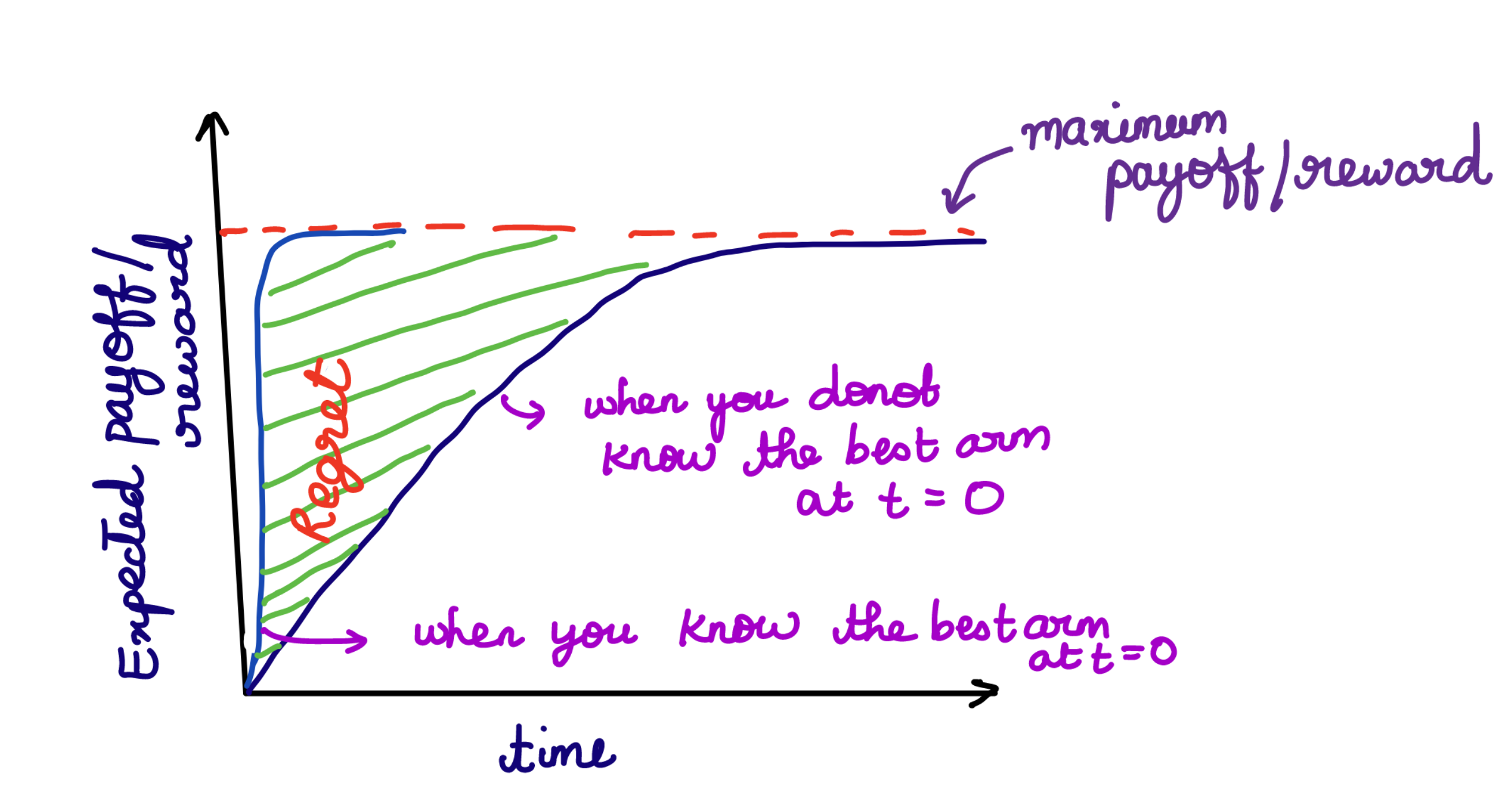
PAC Optimality - PAC stands for Probably Approximately Correct. So there are two parts to this optimality right? “Probably correct” defines if the arm that is picked is optimal or not? and “Approximate correctness” defines how close are we to the optimal action? We also call this the $(\epsilon, \delta)$ PAC optimality. With a probability of $1-\delta$, the solution should be within $\epsilon$ of the best arm.
The goal is to find what is the least number of samples I can pick to achieve PAC optimality given $(\epsilon, \delta)$.
PAC gives us a relative gaurentee which can be denoted in this form below. where $a^*$ is the best arm.

$$ P(q_*(a) \geq q_*(a^*)- \epsilon) \geq (1-\delta) $$

Algorithms to find the best arm!

1. Value function based methods.

$\epsilon$-Greedy Algorithm : As we already saw in the notations, The estimate of the action-value $q_*(a)$ is denoted as $Q_t(a)$. $Q_t$ can be defined as follows,

$$ Q_t = \frac{\text{Sum of rewards when a taken prior to $t$}}{\text{number of times $a$ is taken prior to $t$}} $$

$$ Q_t = \frac{\sum_{i=1}^{t-1}R_i \mathbb{1}_{A_i=a}}{\sum_{i=t}^{t-1}\mathbb{1}_{A_i=a}} $$

where, $\mathbb{1}$ is an indicator function, which means $\mathbb{1} = 1$ if $A_i = a$ else $\mathbb{1} = 0$. In a greedy case, $A_t = \arg \max Q_t(a)$. Greedy forces the algirthm to always exploit the current action. This idea isn’t very efficient as explained above in section-3. The easiest way to tackle this problem is to create an algorithm that will explore for sometime and for sometime it will sample randomly from the action space $A$. This method is called the $\epsilon$-greedy algorithm.
In $\epsilon$-greedy, the algorithm will be greedy with $P(1-\epsilon)$.

$$ = \begin{cases} P(1-\epsilon) & \arg\max Q_t(a) = a^* \\ P(\epsilon) & \text{uniformly sampled from $A$} \end{cases} $$

The problem with $\epsilon$-greedy is that the greedy action gets the bulk of the probability and all the other actions get equally distributed probability.

Soft-max exploration : The problem with $\epsilon$-greedy can be solved by making the probability of picking an action propotional to $Q$.

$$ P(a_t = a) = \frac{Q_t(a)}{\sum_{b=1}^{n}Q_t(b)} $$

Problem with the above equation is that you can end up with a negative probability to pick an action. To encompass all the options and not have negative probabilities we can re-write the above equation to,

$$ P(a_t=a) = \frac{\exp{\frac{Q_t}{\beta}}}{\exp{\frac{\sum_{n=1}{b}Q_t(b)}{\beta}}} $$

$\beta$ is called the temprature parameter. If $\beta \to \infty$ then all the actions are equiprobable, else $\beta \to 0$ actions are selected similar to the greedy algorithm.
In $\epsilon$ - greedy exploration, let’s take $\epsilon = 0.1$ 90$\%$ of the time the algorithm is taking the optimal action and 10 $\%$ of the time it is behaving randomly. To assure some kind of asymptotic correctness, that is we want to make sure after some time the algorithm is only using $q_*$. We can achieve this by cooling down $\epsilon$ gradually.
A food for thought, if you have a stationary distribution from which rewards are sampled all that we discussed makes sense. Suppose an arm is pulled 1000 times, the effect of the reward on the 1001th sample will be very very small. Hint - Can you adjust rewards to give more weight to the recent rewards? If you are interested to read you can refer to page no. 32 and 33 from the book.

Fig:2 Average Regret vs Time

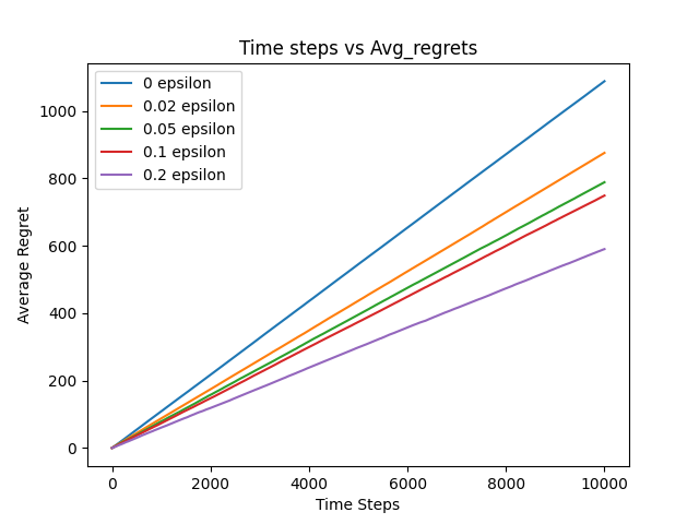
Looking at the above plot can you make deductions about the asymptotic correctness and the regret optimality of the algorithm?

2. Upper Confidence Bounds (UCB-1)

The $\epsilon$-greedy algorithm selects the non-greedy actions indiscriminately. It would be better if we could select among the non-greedy actions according to their potential for actually being optimal, taking how close the value estimates are to the maximal value function and the uncertainities in those estimates.

Let’s first look at the psuedo code of UCB-1 :

$\text{There are $k$-arms, $N$ is discrete time.}$
$\text{$Q(A)$ is the expectation of pulling an arm A}$
Initialize by pulling each arm atleast once.
loop starts:
$\text{Play arm j that maximizes} \arg \max _j Q(j) + \sqrt{\frac{2\ln n}{n_j}}$

The square root term is a measure of uncertainity or variance in the estimate of $Q(a)$. Each time an action $a$ is selected the uncertainity is reduced, because $n_j$ is in the denominator and as number of times you play the $jth$ arm is played increases uncertainity term decreases. On the other end, each time you select a new arm, $n$ increases therfore increasing the uncertainity.
The natural logrithm in the numerator basically means that the increase in uncertainity gets smaller over time. The algorithm facilitates all the actions to be selected but eventually, actions with lower value estimates or that have already been selcted more frequently will be selected with decreasing frequency over time.

What does the UCB therorem state with regards to regret optimality? I am just gonna state the theorem as part of the blog if you are interested you can watch this video.

Theorem : for $k > 0$, if UCB-1 is run on $k$-arms having arbitary reward distribution between $[0, 1]$, then it is expected regret after any number of $n$ plays is at most equal to $8 \sum_{i:q_*(i)<q_*(a^*)}(\frac{\ln n}{\Delta_i}) + (1+\frac{\pi^2}{3}) (\sum_{j=1}^{k} \Delta_j)$ where $\Delta_i = q_*(a^*)-q_*(i)$.
There are many random numbers in that equation that triggers a question on how you arrive at those particular numbers? The video I have linked derives the proof to this theorem using Chernoff-Hoffding bounds also known as large deivation bounds or concentration bounds. (The algorithm is called UCB-1, because there are a lot of variations of UCB and the vanilla UCB is called UCB-1)

Now, UCB-1 also has it’s own set of problems. It is difficult to extend UCB-1 to a more general RL problem for these two major reasons.

It is very complicated to extend UCB-1 to a non-stationary problem.
It is also very difficult to deal with larger state spaces, particularly when using function approximation.

Fig:3 Average Regret vs Time

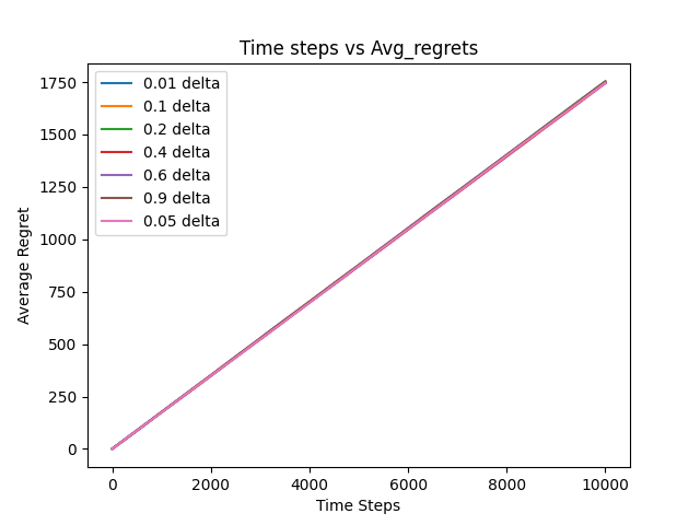
Looking at the above plot can you make deductions about the asymptotic correctness and the regret optimality of the algorithm?

The code for both these algorithms can be found in my git repo.

Conclusion

Right, So it was a longer post than I expected. I had a lot of fun revising all my notes and going through the textbook while writing this blog, I hope you also have the same amount of fun reading this. The MAB problem is just a very small introduction to the full-RL problem. If you noticed in the algorithms we discussed, the actions actually don’t have any consequences or we have not considered a “state propogation model” for the MAB problem. Which is far from the truth in reality, in full RL problems we consider what happens when you take an action and how it affects the state and what are the long-term consequences of taking an action. I am hoping to write atleast one more blog on some basics of RL. Later I will be attempting to implement some papers and write about them.